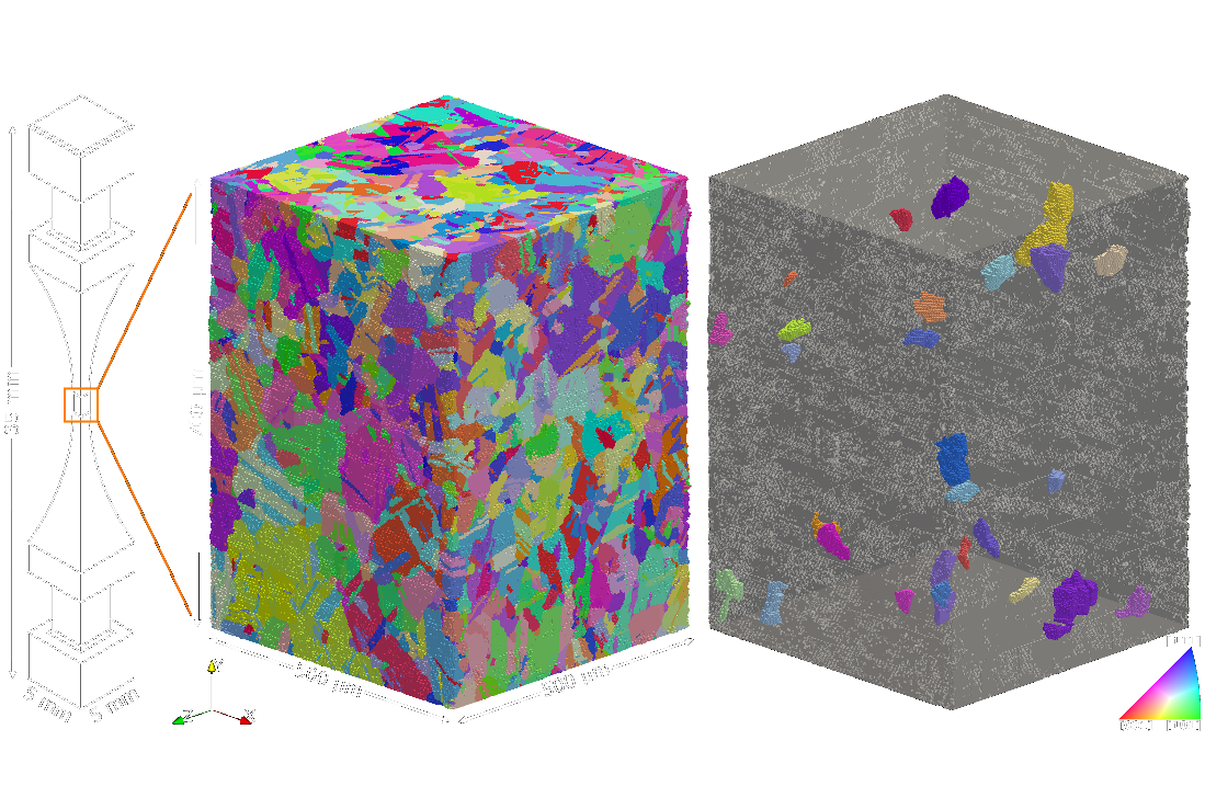
AFRL Challenge
A research challenge in which my team won the top performer award for most accurate microscale structure-to-properties predictions
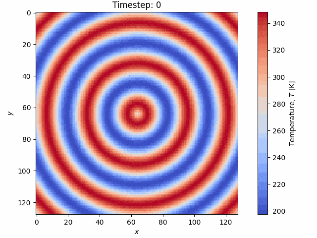
Learn moreThe goal of this project was to solve the anisotropic heat equation using fast Fourier transforms (FFTs) using a graphics processing unit (GPU). The heat equation is a parabolic partial differential equation with the following form: $$\rho c_p \frac{\partial T(\boldsymbol{x})}{\partial t} = \nabla \cdot (k(\boldsymbol x) \nabla T(\boldsymbol x)) + \dot{q}_\mathrm{V}(\boldsymbol x),$$ where \(T\) is the temperature, \(\boldsymbol{x}\) is the spatial position, \(\rho\) is the density, \(c_p\) is the specific heat capacity, \(k\) is the thermal conductivity, and \(\dot{q}_\mathrm{V}\) is the volumetric heat source. The main idea behind solving the heat equation with FFTs is that derivatives in real space become a multiplication by the spatial frequency in Fourier space. We leverage this to compute all the spatial derivatives required for the operators \(\nabla^2 T(\boldsymbol x)\) (homogeneous case) and/or \(\nabla \cdot (k(\boldsymbol x) \nabla T(\boldsymbol x))\) (heterogeneous case) that appears in the heat equation. Once we compute these, the problem becomes a simple ODE that we can integrate using any time-integration technique, of which we use forward Euler and 4th-order Runge-Kutta. At the core of the program, we are simply just performing FFTs, IFFTs, and local point-wise operations in the correct sequence to compute the right-hand side of the heat equation. In the case of heterogeneous materials properties where \(k\) varies in space, the solution is more complicated and takes the following form: $$\rho c_p \frac{\partial T(\boldsymbol x)}{\partial t} = \mathcal{F}^{-1}\Bigl[i \boldsymbol \xi \cdot \mathcal{F}\bigl(k(\boldsymbol x) \mathcal{F}^{-1}[i \boldsymbol \xi \mathcal{F}(T(\boldsymbol x))]\bigr)\Bigr] + \dot{q}_\mathrm{V}(\boldsymbol x),$$ where \(\mathcal F\) denotes a Fourier transform, \(\mathcal F^{-1}\) denotes an inverse Fourier transform, and \(\boldsymbol \xi\) is the spatial frequency vector. In the case that \(k\) is constant, the solution is simpler, easier, and faster to compute than the heterogeneous case: $$\frac{\partial T(\boldsymbol x)}{\partial t} = \frac{\dot{q}_\mathrm{V}(\boldsymbol x)}{\rho c_p} - \frac{k}{\rho c_p} \mathcal{F}^{-1}\Bigl[\|\boldsymbol \xi\|^2_2 \widehat{T}\Bigr](\boldsymbol x),$$ where \(\widehat{T}\) denotes the Fourier transform of \(T\). Once we evaluate the right-hand side of the above equations, we are left with a simple ODE that we can solve with any numerical integration method. Here we use the explicit Euler or explicit 4th-order Runge-Kutta methods. For explicit Euler integration with an isotropic conductivity field, we compute the temperature at time step \(n+1\) as follows: $$T^{(n+1)}(\boldsymbol x) = T^{(n)}(\boldsymbol x) + \left[\frac{\dot{q}_\mathrm{V}(\boldsymbol x)}{\rho c_p} - k\mathcal{F}^{-1}\Bigl[\|\boldsymbol \xi\|^2_2 \widehat{T}^{(n)}\Bigr](\boldsymbol x)\right] \frac{\Delta t}{\rho c_p}.$$ The extension for the 4th-order Runge-Kutta method or for anisotropic conductivity fields is similar. This general solution method using FFTs is less flexible than finite-difference methods as periodic boundary conditions are strictly enforced, but is much faster as a result.
The implementation of the above is done in CUDA and C++ using the highly optimized FFTW and cufft libaries, for the CPU and GPU, respectively. An example simulation from the code is shown below on a \(256 \times 256\) grid with a heterogeneous thermal conductivity field \(k(\boldsymbol x)\):
The code is publicly available on GitHub and is written in C++ and CUDA.
Both a CPU and GPU version are provided, and plotting is performed externally in Python.
https://github.com/cartercocke/Heat-Equation-FFT-GPU
A research challenge in which my team won the top performer award for most accurate microscale structure-to-properties predictions
Learn more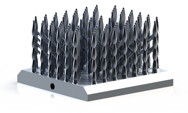
My team's competition-winning natural convection heat sink design for the 2021 ASME/IEEE Heat Sink Design Challenge
Learn more